티스토리 뷰
https://www.kaggle.com/code/ryanholbrook/a-single-neuron
A Single Neuron
Explore and run machine learning code with Kaggle Notebooks | Using data from DL Course Data
www.kaggle.com
Welcome to Deep Learning!
Welcome to Kaggle's Introduction to Deep Learning course! You're about to learn all you need to get started building your own deep neural networks. Using Keras and Tensorflow you'll learn how to:
- create a fully-connected neural network architecture
- apply neural nets to two classic ML problems: regression and classification
- train neural nets with stochastic gradient descent, and
- improve performance with dropout, batch normalization, and other techniques
The tutorials will introduce you to these topics with fully-worked examples, and then in the exercises, you'll explore these topics in more depth and apply them to real-world datasets.
Let's get started!
What is Deep Learning?
Some of the most impressive advances in artificial intelligence in recent years have been in the field of deep learning. Natural language translation, image recognition, and game playing are all tasks where deep learning models have neared or even exceeded human-level performance.
So what is deep learning? Deep learning is an approach to machine learning characterized by deep stacks of computations. This depth of computation is what has enabled deep learning models to disentangle the kinds of complex and hierarchical patterns found in the most challenging real-world datasets.
Through their power and scalability neural networks have become the defining model of deep learning. Neural networks are composed of neurons, where each neuron individually performs only a simple computation. The power of a neural network comes instead from the complexity of the connections these neurons can form.
The Linear Unit
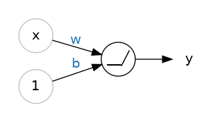
So let's begin with the fundamental component of a neural network: the individual neuron. As a diagram, a neuron (or unit) with one input looks like:
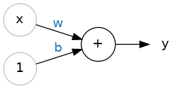
The input is x. Its connection to the neuron has a weight which is w. Whenever a value flows through a connection, you multiply the value by the connection's weight. For the input x, what reaches the neuron is w * x. A neural network "learns" by modifying its weights.
The b is a special kind of weight we call the bias. The bias doesn't have any input data associated with it; instead, we put a 1 in the diagram so that the value that reaches the neuron is just b (since 1 * b = b). The bias enables the neuron to modify the output independently of its inputs.
The y is the value the neuron ultimately outputs. To get the output, the neuron sums up all the values it receives through its connections. This neuron's activation is y = w * x + b, or as a formula 𝑦=𝑤𝑥+𝑏�=��+�.
Does the formula 𝑦=𝑤𝑥+𝑏�=��+� look familiar?
It's an equation of a line! It's the slope-intercept equation, where 𝑤� is the slope and 𝑏� is the y-intercept.
Example - The Linear Unit as a Model
Though individual neurons will usually only function as part of a larger network, it's often useful to start with a single neuron model as a baseline. Single neuron models are linear models.
Let's think about how this might work on a dataset like 80 Cereals. Training a model with 'sugars' (grams of sugars per serving) as input and 'calories' (calories per serving) as output, we might find the bias is b=90 and the weight is w=2.5. We could estimate the calorie content of a cereal with 5 grams of sugar per serving like this:
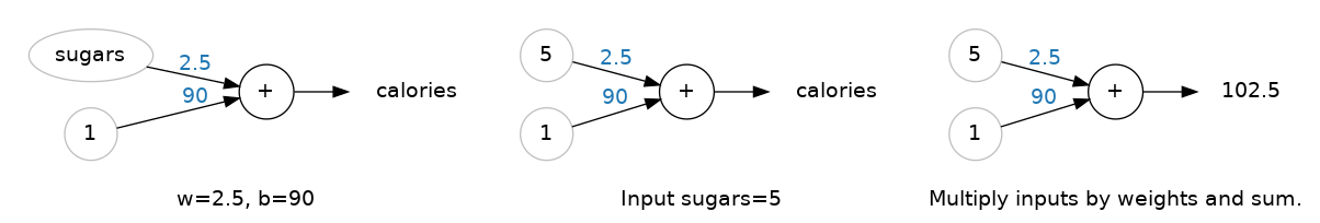
And, checking against our formula, we have 𝑐𝑎𝑙𝑜𝑟𝑖𝑒𝑠=2.5×5+90=102.5��������=2.5×5+90=102.5, just like we expect.
Multiple Inputs
The 80 Cereals dataset has many more features than just 'sugars'. What if we wanted to expand our model to include things like fiber or protein content? That's easy enough. We can just add more input connections to the neuron, one for each additional feature. To find the output, we would multiply each input to its connection weight and then add them all together.
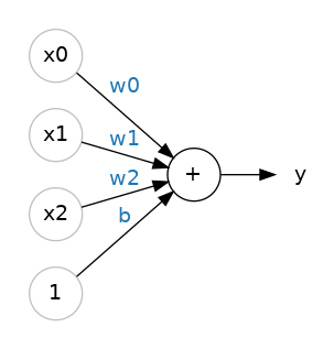
The formula for this neuron would be 𝑦=𝑤0𝑥0+𝑤1𝑥1+𝑤2𝑥2+𝑏�=�0�0+�1�1+�2�2+�. A linear unit with two inputs will fit a plane, and a unit with more inputs than that will fit a hyperplane.
Linear Units in Keras
The easiest way to create a model in Keras is through keras.Sequential, which creates a neural network as a stack of layers. We can create models like those above using a dense layer (which we'll learn more about in the next lesson).
We could define a linear model accepting three input features ('sugars', 'fiber', and 'protein') and producing a single output ('calories') like so:
from tensorflow import keras
from tensorflow.keras import layers

# Create a network with 1 linear unit
model = keras.Sequential([
    layers.Dense(units=1, input_shape=[3])
])
With the first argument, units, we define how many outputs we want. In this case we are just predicting 'calories', so we'll use units=1.
With the second argument, input_shape, we tell Keras the dimensions of the inputs. Setting input_shape=[3] ensures the model will accept three features as input ('sugars', 'fiber', and 'protein').
This model is now ready to be fit to training data!
Why is input_shape a Python list?
The data we'll use in this course will be tabular data, like in a Pandas dataframe. We'll have one input for each feature in the dataset. The features are arranged by column, so we'll always have input_shape=[num_columns]. The reason Keras uses a list here is to permit use of more complex datasets. Image data, for instance, might need three dimensions: [height, width, channels].
Deep Neural Networks
Explore and run machine learning code with Kaggle Notebooks | Using data from DL Course Data
www.kaggle.com
Introduction
In this lesson we're going to see how we can build neural networks capable of learning the complex kinds of relationships deep neural nets are famous for.
The key idea here is modularity, building up a complex network from simpler functional units. We've seen how a linear unit computes a linear function -- now we'll see how to combine and modify these single units to model more complex relationships.
우리는 심층 신경망이 유명한 복잡한 종류의 관계를 학습할 수 있는 신경망을 구축할 수 있는 방법을 살펴보겠습니다.
여기서 핵심 아이디어는 모듈성, 즉 단순한 기능 단위로 복잡한 네트워크를 구축하는 것입니다. 선형 단위가 선형 함수를 계산하는 방법을 살펴보았습니다. 이제 이러한 단일 단위를 결합하고 수정하여 보다 복잡한 관계를 모델링하는 방법을 살펴보겠습니다.
Layers
Neural networks typically organize their neurons into layers. When we collect together linear units having a common set of inputs we get a dense layer.

A dense layer of two linear units receiving two inputs and a bias.
You could think of each layer in a neural network as performing some kind of relatively simple transformation. Through a deep stack of layers, a neural network can transform its inputs in more and more complex ways. In a well-trained neural network, each layer is a transformation getting us a little bit closer to a solution.
Many Kinds of Layers
A "layer" in Keras is a very general kind of thing. A layer can be, essentially, any kind of data transformation. Many layers, like the convolutional and recurrent layers, transform data through use of neurons and differ primarily in the pattern of connections they form. Others though are used for feature engineering or just simple arithmetic. There's a whole world of layers to discover -- check them out!
레이어
신경망은 일반적으로 뉴런을 레이어로 구성합니다. 공통 입력 세트를 갖는 선형 단위를 함께 모으면 조밀한 레이어가 생성됩니다.
입력 레이어에 있는 세 개의 원이 밀집 레이어의 두 원에 연결된 스택입니다.
두 개의 입력과 바이어스를 받는 두 개의 선형 유닛으로 구성된 조밀한 레이어입니다.
신경망의 각 계층은 비교적 간단한 변환을 수행하는 것으로 생각할 수 있습니다. 심층적인 레이어 스택을 통해 신경망은 입력을 점점 더 복잡한 방식으로 변환할 수 있습니다. 잘 훈련된 신경망에서 각 계층은 솔루션에 조금 더 가까워지는 변환입니다.
다양한 종류의 레이어
Keras의 "레이어"는 매우 일반적인 종류의 것입니다. 레이어는 기본적으로 모든 종류의 데이터 변환이 될 수 있습니다. 컨벌루션 및 순환 레이어와 같은 많은 레이어는 뉴런을 사용하여 데이터를 변환하며 주로 형성하는 연결 패턴이 다릅니다. 그러나 다른 것들은 기능 엔지니어링이나 단순한 산술에 사용됩니다. 발견할 수 있는 레이어의 세계가 무궁무진합니다. 확인해 보세요!
The Activation Function
It turns out, however, that two dense layers with nothing in between are no better than a single dense layer by itself. Dense layers by themselves can never move us out of the world of lines and planes. What we need is something nonlinear. What we need are activation functions.
활성화 기능
그러나 사이에 아무것도 없는 두 개의 Dense 레이어는 그 자체로 하나의 Dense 레이어보다 나을 것이 없다는 것이 밝혀졌습니다. 밀도가 높은 레이어만으로는 우리를 선과 면의 세계에서 결코 벗어날 수 없습니다. 우리에게 필요한 것은 비선형적인 것입니다. 우리에게 필요한 것은 활성화 함수입니다.
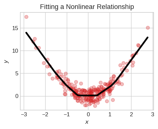
An activation function is simply some function we apply to each of a layer's outputs (its activations). The most common is the rectifier function 𝑚𝑎𝑥(0,𝑥)���(0,�).
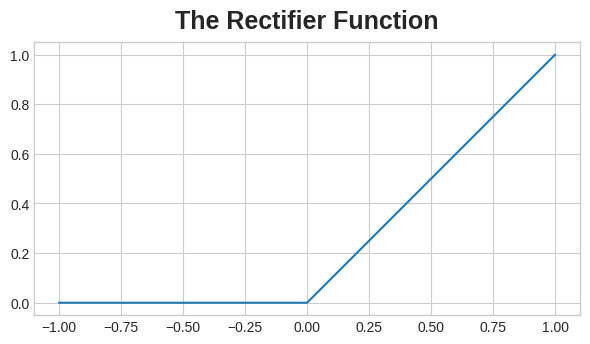
The rectifier function has a graph that's a line with the negative part "rectified" to zero. Applying the function to the outputs of a neuron will put a bend in the data, moving us away from simple lines.
When we attach the rectifier to a linear unit, we get a rectified linear unit or ReLU. (For this reason, it's common to call the rectifier function the "ReLU function".) Applying a ReLU activation to a linear unit means the output becomes max(0, w * x + b), which we might draw in a diagram like:
정류기 함수에는 음수 부분이 0으로 "수정된" 선인 그래프가 있습니다. 뉴런의 출력에 함수를 적용하면 데이터가 구부러져 단순한 선에서 멀어지게 됩니다.
정류기를 선형 장치에 연결하면 정류된 선형 장치 또는 ReLU가 생성됩니다. (이런 이유로 정류 함수를 "ReLU 함수"라고 부르는 것이 일반적입니다.) ReLU 활성화를 선형 단위에 적용하면 출력이 max(0, w * x + b)가 됨을 의미하며, 이를 다음과 같은 다이어그램으로 그릴 수 있습니다. :
Stacking Dense Layers
Now that we have some nonlinearity, let's see how we can stack layers to get complex data transformations.
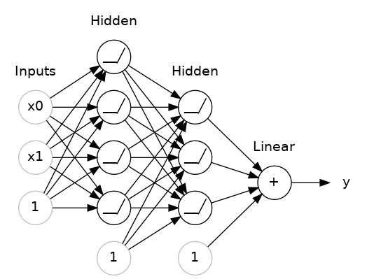
The layers before the output layer are sometimes called hidden since we never see their outputs directly.
Now, notice that the final (output) layer is a linear unit (meaning, no activation function). That makes this network appropriate to a regression task, where we are trying to predict some arbitrary numeric value. Other tasks (like classification) might require an activation function on the output.
Building Sequential Models
The Sequential model we've been using will connect together a list of layers in order from first to last: the first layer gets the input, the last layer produces the output. This creates the model in the figure above:
from tensorflow import keras
from tensorflow.keras import layers

model = keras.Sequential([
    # the hidden ReLU layers
    layers.Dense(units=4, activation='relu', input_shape=[2]),
    layers.Dense(units=3, activation='relu'),
    # the linear output layer
    layers.Dense(units=1),
])
Be sure to pass all the layers together in a list, like [layer, layer, layer, ...], instead of as separate arguments. To add an activation function to a layer, just give its name in the activation argument.
03 SGD
Introduction
In the first two lessons, we learned how to build fully-connected networks out of stacks of dense layers. When first created, all of the network's weights are set randomly -- the network doesn't "know" anything yet. In this lesson we're going to see how to train a neural network; we're going to see how neural networks learn.
처음 두 강의에서는 밀집된 레이어 스택으로 완전히 연결된 네트워크를 구축하는 방법을 배웠습니다. 처음 생성될 때 네트워크의 모든 가중치는 무작위로 설정됩니다. 즉, 네트워크는 아직 아무것도 "알지" 못합니다. 이번 강의에서는 신경망을 훈련하는 방법을 살펴보겠습니다. 우리는 신경망이 어떻게 학습하는지 살펴보겠습니다.
As with all machine learning tasks, we begin with a set of training data. Each example in the training data consists of some features (the inputs) together with an expected target (the output). Training the network means adjusting its weights in such a way that it can transform the features into the target. In the 80 Cereals dataset, for instance, we want a network that can take each cereal's 'sugar', 'fiber', and 'protein' content and produce a prediction for that cereal's 'calories'. If we can successfully train a network to do that, its weights must represent in some way the relationship between those features and that target as expressed in the training data.
모든 기계 학습 작업과 마찬가지로 훈련 데이터 세트로 시작합니다. 훈련 데이터의 각 예는 예상 목표(출력)와 함께 일부 기능(입력)으로 구성됩니다. 네트워크를 훈련한다는 것은 특성을 목표로 변환할 수 있는 방식으로 가중치를 조정하는 것을 의미합니다. 예를 들어 80가지 곡물 데이터세트에서 우리는 각 곡물의 '설탕', '섬유질' 및 '단백질' 함량을 가져와 해당 곡물의 '칼로리'에 대한 예측을 생성할 수 있는 네트워크를 원합니다. 이를 수행하도록 네트워크를 성공적으로 훈련할 수 있다면 해당 가중치는 훈련 데이터에 표현된 해당 기능과 대상 간의 관계를 어떤 방식으로든 나타내야 합니다.모든 기계 학습 작업과 마찬가지로 훈련 데이터 세트로 시작합니다. 훈련 데이터의 각 예는 예상 목표(출력)와 함께 일부 기능(입력)으로 구성됩니다. 네트워크를 훈련한다는 것은 특성을 목표로 변환할 수 있는 방식으로 가중치를 조정하는 것을 의미합니다. 예를 들어 80가지 곡물 데이터세트에서 우리는 각 곡물의 '설탕', '섬유질' 및 '단백질' 함량을 가져와 해당 곡물의 '칼로리'에 대한 예측을 생성할 수 있는 네트워크를 원합니다. 이를 수행하도록 네트워크를 성공적으로 훈련할 수 있다면 해당 가중치는 훈련 데이터에 표현된 해당 기능과 대상 간의 관계를 어떤 방식으로든 나타내야 합니다.
In addition to the training data, we need two more things:
- A "loss function" that measures how good the network's predictions are.
- An "optimizer" that can tell the network how to change its weights.
훈련 데이터 외에도 두 가지가 더 필요합니다.
네트워크의 예측이 얼마나 좋은지 측정하는 "손실 함수"입니다.
네트워크에 가중치를 변경하는 방법을 알려줄 수 있는 "최적화 프로그램"입니다.
The Loss Function
We've seen how to design an architecture for a network, but we haven't seen how to tell a network what problem to solve. This is the job of the loss function.
The loss function measures the disparity between the the target's true value and the value the model predicts.
우리는 네트워크 아키텍처를 설계하는 방법을 살펴봤지만 네트워크에 어떤 문제를 해결해야 하는지 알려주는 방법은 보지 못했습니다. 이것이 손실 함수의 역할입니다.
손실 함수는 대상의 실제 값과 모델이 예측하는 값 간의 차이를 측정합니다.
Different problems call for different loss functions. We have been looking at regression problems, where the task is to predict some numerical value -- calories in 80 Cereals, rating in Red Wine Quality. Other regression tasks might be predicting the price of a house or the fuel efficiency of a car.
A common loss function for regression problems is the mean absolute error or MAE. For each prediction y_pred, MAE measures the disparity from the true target y_true by an absolute difference abs(y_true - y_pred).
문제마다 다른 손실 함수가 필요합니다. 우리는 레드 와인 품질 등급인 시리얼 80개의 칼로리와 같은 수치 값을 예측하는 것이 임무인 회귀 문제를 살펴보았습니다. 다른 회귀 작업으로는 주택 가격이나 자동차의 연비를 예측하는 것이 있을 수 있습니다.
회귀 문제에 대한 일반적인 손실 함수는 평균 절대 오차(MAE)입니다. 각 예측 y_pred에 대해 MAE는 절대 차이 abs(y_true - y_pred)로 실제 목표 y_true와의 차이를 측정합니다.
The total MAE loss on a dataset is the mean of all these absolute differences.
Besides MAE, other loss functions you might see for regression problems are the mean-squared error (MSE) or the Huber loss (both available in Keras).
During training, the model will use the loss function as a guide for finding the correct values of its weights (lower loss is better). In other words, the loss function tells the network its objective.
The Optimizer - Stochastic Gradient Descent
We've described the problem we want the network to solve, but now we need to say how to solve it. This is the job of the optimizer. The optimizer is an algorithm that adjusts the weights to minimize the loss.
Virtually all of the optimization algorithms used in deep learning belong to a family called stochastic gradient descent. They are iterative algorithms that train a network in steps. One step of training goes like this:
- Sample some training data and run it through the network to make predictions.
- Measure the loss between the predictions and the true values.
- Finally, adjust the weights in a direction that makes the loss smaller.
Then just do this over and over until the loss is as small as you like (or until it won't decrease any further.)
Each iteration's sample of training data is called a minibatch (or often just "batch"), while a complete round of the training data is called an epoch. The number of epochs you train for is how many times the network will see each training example.
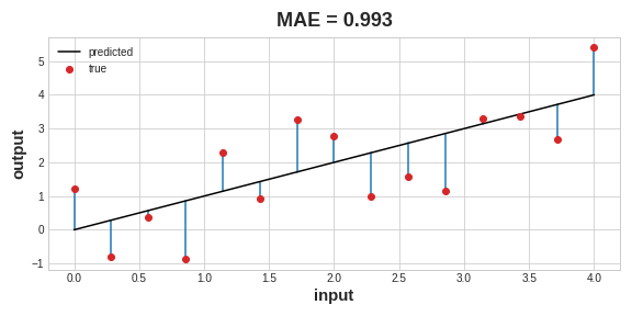
The animation shows the linear model from Lesson 1 being trained with SGD. The pale red dots depict the entire training set, while the solid red dots are the minibatches. Every time SGD sees a new minibatch, it will shift the weights (w the slope and b the y-intercept) toward their correct values on that batch. Batch after batch, the line eventually converges to its best fit. You can see that the loss gets smaller as the weights get closer to their true values.
Learning Rate and Batch Size
Notice that the line only makes a small shift in the direction of each batch (instead of moving all the way). The size of these shifts is determined by the learning rate. A smaller learning rate means the network needs to see more minibatches before its weights converge to their best values.
The learning rate and the size of the minibatches are the two parameters that have the largest effect on how the SGD training proceeds. Their interaction is often subtle and the right choice for these parameters isn't always obvious. (We'll explore these effects in the exercise.)
Fortunately, for most work it won't be necessary to do an extensive hyperparameter search to get satisfactory results. Adam is an SGD algorithm that has an adaptive learning rate that makes it suitable for most problems without any parameter tuning (it is "self tuning", in a sense). Adam is a great general-purpose optimizer.
Adding the Loss and Optimizer
After defining a model, you can add a loss function and optimizer with the model's compile method:
model.compile(
    optimizer="adam",
    loss="mae",
)
Notice that we are able to specify the loss and optimizer with just a string. You can also access these directly through the Keras API -- if you wanted to tune parameters, for instance -- but for us, the defaults will work fine.
What's In a Name?
The gradient is a vector that tells us in what direction the weights need to go. More precisely, it tells us how to change the weights to make the loss change fastest. We call our process gradient descent because it uses the gradient to descend the loss curve towards a minimum. Stochastic means "determined by chance." Our training is stochastic because the minibatches are random samples from the dataset. And that's why it's called SGD!
Example - Red Wine Quality
Now we know everything we need to start training deep learning models. So let's see it in action! We'll use the Red Wine Quality dataset.
This dataset consists of physiochemical measurements from about 1600 Portuguese red wines. Also included is a quality rating for each wine from blind taste-tests. How well can we predict a wine's perceived quality from these measurements?
We've put all of the data preparation into this next hidden cell. It's not essential to what follows so feel free to skip it. One thing you might note for now though is that we've rescaled each feature to lie in the interval [0,1][0,1]. As we'll discuss more in Lesson 5, neural networks tend to perform best when their inputs are on a common scale.
| 10.8 | 0.470 | 0.43 | 2.10 | 0.171 | 27.0 | 66.0 | 0.99820 | 3.17 | 0.76 | 10.8 | 6 |
| 8.1 | 0.820 | 0.00 | 4.10 | 0.095 | 5.0 | 14.0 | 0.99854 | 3.36 | 0.53 | 9.6 | 5 |
| 9.1 | 0.290 | 0.33 | 2.05 | 0.063 | 13.0 | 27.0 | 0.99516 | 3.26 | 0.84 | 11.7 | 7 |
| 10.2 | 0.645 | 0.36 | 1.80 | 0.053 | 5.0 | 14.0 | 0.99820 | 3.17 | 0.42 | 10.0 | 6 |
How many inputs should this network have? We can discover this by looking at the number of columns in the data matrix. Be sure not to include the target ('quality') here -- only the input features.
print(X_train.shape)
(1119, 11)
Eleven columns means eleven inputs.
We've chosen a three-layer network with over 1500 neurons. This network should be capable of learning fairly complex relationships in the data.
from tensorflow import keras
from tensorflow.keras import layers

model = keras.Sequential([
    layers.Dense(512, activation='relu', input_shape=[11]),
    layers.Dense(512, activation='relu'),
    layers.Dense(512, activation='relu'),
    layers.Dense(1),
])
Deciding the architecture of your model should be part of a process. Start simple and use the validation loss as your guide. You'll learn more about model development in the exercises.
After defining the model, we compile in the optimizer and loss function.
model.compile(
    optimizer='adam',
    loss='mae',
)
Now we're ready to start the training! We've told Keras to feed the optimizer 256 rows of the training data at a time (the batch_size) and to do that 10 times all the way through the dataset (the epochs).
history = model.fit(
    X_train, y_train,
    validation_data=(X_valid, y_valid),
    batch_size=256,
    epochs=10,
)
Epoch 1/10
5/5 [==============================] - 1s 66ms/step - loss: 0.2470 - val_loss: 0.1357
Epoch 2/10
5/5 [==============================] - 0s 21ms/step - loss: 0.1349 - val_loss: 0.1231
Epoch 3/10
5/5 [==============================] - 0s 23ms/step - loss: 0.1181 - val_loss: 0.1173
Epoch 4/10
5/5 [==============================] - 0s 21ms/step - loss: 0.1117 - val_loss: 0.1066
Epoch 5/10
5/5 [==============================] - 0s 22ms/step - loss: 0.1071 - val_loss: 0.1028
Epoch 6/10
5/5 [==============================] - 0s 20ms/step - loss: 0.1049 - val_loss: 0.1050
Epoch 7/10
5/5 [==============================] - 0s 20ms/step - loss: 0.1035 - val_loss: 0.1009
Epoch 8/10
5/5 [==============================] - 0s 20ms/step - loss: 0.1019 - val_loss: 0.1043
Epoch 9/10
5/5 [==============================] - 0s 19ms/step - loss: 0.1005 - val_loss: 0.1035
Epoch 10/10
5/5 [==============================] - 0s 20ms/step - loss: 0.1011 - val_loss: 0.0977
You can see that Keras will keep you updated on the loss as the model trains.
Often, a better way to view the loss though is to plot it. The fit method in fact keeps a record of the loss produced during training in a History object. We'll convert the data to a Pandas dataframe, which makes the plotting easy.
import pandas as pd

# convert the training history to a dataframe
history_df = pd.DataFrame(history.history)
# use Pandas native plot method
history_df['loss'].plot();
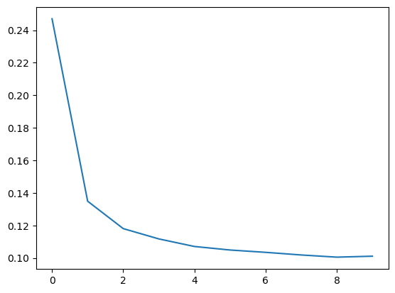
Notice how the loss levels off as the epochs go by. When the loss curve becomes horizontal like that, it means the model has learned all it can and there would be no reason continue for additional epochs.
'딥러닝' 카테고리의 다른 글
| Dropout and Batch Normalization (0) | 2023.10.30 |
|---|---|
| Overfitting and Underfitting (0) | 2023.10.30 |
| self-study road map (0) | 2023.10.27 |
| Getting Started with Deep Learning (0) | 2023.10.27 |
| GAN (0) | 2023.10.27 |
- Total
- Today
- Yesterday
- 자바
- LECTURE
- linkedin-skill-assessments-quizzes
- 기본
- Neo4j
- Shell
- ML
- MachineLearning
- pytorch
- 통계
- extract archive multiple files
- 알고리즘
- LeetCode
- quiz
- tag hello
- Paper
- nvidia #gan
- mongodb
- amazon
- 파이썬
- geometry
| 일 | 월 | 화 | 수 | 목 | 금 | 토 |
|---|---|---|---|---|---|---|
| 1 | 2 | 3 | 4 | 5 | 6 | |
| 7 | 8 | 9 | 10 | 11 | 12 | 13 |
| 14 | 15 | 16 | 17 | 18 | 19 | 20 |
| 21 | 22 | 23 | 24 | 25 | 26 | 27 |
| 28 | 29 | 30 | 31 |